Matrix Contribution Correlation Comparison

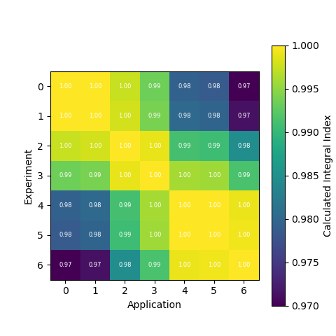
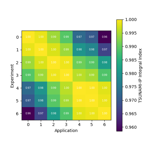
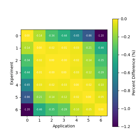
This example demonstrates how to generate a matrix comparison plot for the contribution correlation method (described in Matrix of Contribution Correlation Plots and Perturbation Correlation Plots). This example compares the calculated correlation correlation coefficient to the TSUNAMI-IP calculated \(c_k\) value for a set of SDFs computed from the HMF series of critical experiments [Bess2019].

Getting TSUNAMI-IP \(c_k\) Values

First, we need to get the TSUNAMI-IP \(c_k\) values for the experiment and application SDFs we want to compare. We can do this by using the tsunami_ip_utils.integral_indices.get_integral_indices() function, as shown in Reading Integral Indices.

from tsunami_ip_utils.integral_indices import get_integral_indices
from paths import EXAMPLES

application_sdfs = [ EXAMPLES / 'data' / 'example_sdfs' / 'HMF' / f'HEU-MET-FAST-003-00{i}.sdf' for i in range(1, 8) ]
experiment_sdfs = application_sdfs

# Get the TSUNAMI-IP integral indices
coverx_library = '56groupcov7.1'
integral_indices = get_integral_indices(application_sdfs, experiment_sdfs, coverx_library=coverx_library)
c_k = integral_indices['c_k']

Nuclide-Wise Comparison

Variance Contributions

First we show a comparison of the calculated correlation coefficient using the contribution correlation method with nuclide-wise variance contributions to the TSUNAMI-IP \(c_k\) values. To generate this comparison, we just have to specify the correct method, which in this case is 'variance_contributions_nuclide'.

from tsunami_ip_utils.comparisons import correlation_comparison

labels = {
    'applications': [ application_file.name for application_file in application_sdfs ],
    'experiments': [ experiment_file.name for experiment_file in experiment_sdfs ],
}
comparisons, fig = correlation_comparison(
    integral_index_matrix=c_k,
    integral_index_name='c_k',
    application_files=application_sdfs,
    experiment_files=experiment_sdfs,
    method='variance_contributions_nuclide',
    matrix_plot_kwargs={'labels': labels},
)
fig.show()

- Zoom Out + Zoom In

Uncertainty Contributions

We can also generate a comparison using the contribution correlation method with the uncertainty contributions

comparisons, fig = correlation_comparison(
    integral_index_matrix=c_k,
    integral_index_name='c_k',
    application_files=application_sdfs,
    experiment_files=experiment_sdfs,
    method='uncertainty_contributions_nuclide',
)
fig.show()

- Zoom Out + Zoom In

We can also generate an image of the comparison

comparisons, fig = correlation_comparison(
    integral_index_matrix=c_k,
    integral_index_name='c_k',
    application_files=application_sdfs,
    experiment_files=experiment_sdfs,
    method='uncertainty_contributions_nuclide',
)
fig.to_image( EXAMPLES / '_static' / 'contribution_matrix_comparison.png' )

# sphinx_gallery_thumbnail_path = '../../examples/_static/contribution_matrix_comparison.png'

- Zoom Out + Zoom In

Generating a Comparison Heatmap

We can also generate a heatmap of the comparison between the calculated correlation coefficient and the TSUNAMI-IP \(c_k\) values by using the tsunami_ip_utils.viz.generate_heatmap_from_comparison() function.

from tsunami_ip_utils.viz import generate_heatmap_from_comparison

plot_dict = generate_heatmap_from_comparison(comparisons)

print(plot_dict.keys())

• 
• 
• 
• 

dict_keys(['Calculated', 'TSUNAMI-IP', 'Percent Difference'])

The tsunami_ip_utils.viz.generate_heatmap_from_comparison() takes in the comparison dataframe generated by the tsunami_ip_utils.comparisons_correlation_comparison() function and returns a dictionary of matplotlib heatmaps. From the output above you can see that the function contains heatmaps of the calculated value, the TSUNAMI-IP value, and the percent difference between the two. Note that this function was used to generate the plots shown in the technical manual.

fig, axs = plot_dict['Calculated']
fig.show()

fig, axs = plot_dict['TSUNAMI-IP']
fig.show()

fig, axs = plot_dict['Percent Difference']
fig.show()