Investigation of Correlation Methods for use in Criticality Safety
- Author:
Matthew Louis
- Author:
Alex Lang
- Author:
Walid Metwally
Background
In the field of criticality safety, computational methods are used for ensuring subcriticality for processes under normal and credible abnormal conditions. To ensure that these computational methods for ensuring operational safety are reliable, they must be rigorously validated against physical experiments. The American National Institute of Standards (ANSI) outlines the procedure for code validation for criticality safety in ANSI/ANS-8.1 [BB08]. The standard requires that the computational bias for a particular application is well quantified by comparison with experiments within some range of applicability. The standard defines the range of applicability as “the limiting ranges of material compositions, geometric arrangements, neutron energy spectra, and other relevant parameters e.g., heterogeneity, leakage, interaction, absorption, etc. within which the bias of a computational method is established” [BB08] For systems that may lack applicable experiments entirely (e.g., UF6 transportation cylinders [SLMH21]), the standard allows for using trends in the bias to extend the experimental data to the application system.
Historically, this bias trending has required expert judgement about which system characteristics should be used for defining similarity for the trending analysis (neutron spectrum, fuel enrichment, etc.). A key development was the introduction of quantitative similarity metrics based on system sensitivity and nuclear data–induced uncertainty [BRH+04]. The conjecture is that systems will have similar biases if they have similar sensitivity/uncertainty profiles (on a nuclide-reaction group-wise level) because it is thought that the bias is primarily the result of uncertainties in the underlying nuclear data. These similarity indices can then be used with bias trending analysis tools like those provided by the SCALE code sequence VADER [HC22] to provide a quantitative physics–based method for estimating computational bias that does not rely on expert judgement.
Important Similarity Indices
Of the several similarity indices defined by Broadhead et al., [BRH+04] the two prominent indices available in SCALE are \(E\) and \(c_k\) [WL23].
The Sensitivity-Based Similarity Index: \(E\)
The integral index \(E\) is defined solely in terms of the sensitivity profiles (i.e., the set of group-wise \(k_{\text{eff}}\) sensitivities for each nuclide-reaction pair), which may be calculated using standard methods like Contributon-Linked eigenvalue sensitivity/uncertainty estimation via Tracklength importance Characterization (CLUTCH), [Per12] Iterated Fission Probability, [Hur48, Kie09] direct perturbation, and others. Most of these methods are implemented in SCALE’s TSUNAMI-3D sequence [MCR20, PR15]. It was thought that if two systems are similar, their eigenvalue response to perturbations in input nuclear data, or their sensitivity profiles, should be similar. The integral index \(E\) was designed to automate the (often) manual comparisons of sensitivity profiles for each nuclide reaction. To compute an integral index, the sensitivity profiles of two arbitrary systems, A and B, are formed as vectors (where zero sensitivities are assigned to missing nuclides or reactions so that the vectors have compatible lengths) \(\boldsymbol{S}_A\) and \(\boldsymbol{S}_B\), and their normalized vector dot product is taken to be the degree of similarity between system A and system B:
\(E\) is not typically used when predicting bias, however, as it does not incorporate the nuclear data uncertainty. While shared sensitivity to nuclear data indicates an experiment may be applicable, it is not the best predictor of computational bias, which is driven by nuclear data induced uncertainty.
The Uncertainty-Based Similarity Index: \(c_k\)
The most widely used similarity index in criticality safety is \(c_k\). It represents the degree to which nuclear data–induced uncertainties in \(k_{\text{eff}}\) are correlated between two systems [BRH+04]. The \(c_k\) similarity index between systems A and B is given by
where \(\boldsymbol{S}_A\) and \(\boldsymbol{S}_B\) are respectively the sensitivity (row) vectors each of length \(M=G\times P\), where \(P\) represents the total number of (unique) nuclide reaction pairs in the system and application, \(G\) is the number of energy groups, and \(\boldsymbol{C}_{\alpha, \alpha}\) is the nuclear data covariance matrix (with shape \(M\times M\)) defined by
where \(\sigma_i\) represents a single group-wise cross section for a given nuclide-reaction pair and is the smallest unit of nuclear data in a multigroup library. The denominator serves as a normalization factor to ensure that if \(\boldsymbol{S}_A=\boldsymbol{S}_B\) when \(c_k=1\), and if \(\boldsymbol{S}_A=-\boldsymbol{S}_B\), then \(c_k=-1\). This definition is aesthetically similar to that of Pearson’s correlation coefficient between two random variables \(X\) and \(Y\), as in Eq. (2). The only caveat is that the nuclear data covariance matrices can sometimes be problematic [MRH09] and lead to nonphysical results unless certain heuristic rules are applied (i.e., those in the \(\texttt{cov\_fix}\) option) [WL23]. Furthermore there are concerns about the presence of unevaluated cross-section covariances and their impact on similarity [MRH09].
Bias Estimation and Acceptance Criteria
When estimating the computational bias using techniques like the Generalized Linear Least Squares method (GLLSM), or other bias estimation tools with similarity parameters like \(c_k\), a cutoff is generally chosen for the similarity index below which experiments are not included in the bias estimation. From an intuitive perspective, it is unreasonable to expect that experiments that are very dissimilar to the application would provide a useful estimation of the bias, so a cutoff of some sort is necessary. For thermal systems, parametric studies have been performed over the cutoff, and the cutoffs that were found to minimize the bias error were identified [BRH+04]. In addition, the number of experiments needed to obtain a given confidence in the estimated bias was also explored. From these considerations, a \(c_k\) cutoff of \(0.9\) was chosen as a general recommendation [BRH+04] and is commonly used in regulatory guidance, [SMW14] but lower \(c_k\) cutoffs can be used, although they require more experiments to achieve the same confidence in the estimated bias. These criteria are a general heuristic, and optimal \(c_k\) cutoffs depend on the physical parameters of the system and the chosen validation suite as well.
Practical Issues with the Application of Similarity Indices
For many low-enriched, light water applications, the prescriptive \(c_k\geq 0.9\) is not prohibitive, and it allows the practitioner sufficient flexibility when selecting a suite of experiments for code validation. However, the recent interest in high-assay low-enriched uranium (HALEU) has required designing systems (mainly for transportation) for which there is a general lack of applicable experiments [FDAQ+24]. For these applications, practitioners are required to make an estimation of the computational bias, despite having few or no experiments with \(c_k\geq 0.9\). As discussed, there is a complex relationship between the \(c_k\) of included experiments, the number of included experiments, and the quality of the estimated computational bias, so it is not immediately clear how to select experiment suites in these cases. Can practitioners lower the \(c_k\) threshold to get more applicable experiments to achieve a better estimate of the bias, or would including dissimilar experiments provide a poor estimate of the bias and/or violate the assumptions of the bias trending method? Is the heuristic guidance for the \(c_k\) threshold even applicable in this case?
To address these questions, a better understanding of how the underlying nuclear data influences the calculated \(c_k\) could be useful. Broadhead et al. provide a means for calculating the contributions to \(c_k\) on a nuclide- and reaction-specific basis, which can be helpful when determining which nuclides and reactions are driving similarity or dissimilarity. Examination of these contributions can be descriptive and can help inform experiment design because relevant dissimilar isotopes and reactions can be readily identified. As an exploratory effort, other ways of visually representing the contributions to \(c_k\) were explored.
A Correlation Based Approach
To aid in understanding the contributions of individual sensitivities and nuclear data uncertainties necessary in the computation of Eq. (1), visualization tools can be used to graphically inspect the contributors to the integral value. This approach would allow practitioners to interpret the similarity between two systems as the degree to which they are correlated and would allow outliers to be easily identified. In addition, other traditional statistical measures of correlation could be used to asses similarity, such as the Spearman or Kendall rank correlation coefficient, which give different weights to various aspects of the constituent datasets, and they could also be useful as similarity indices, though these applications are not explored in this work.
The Correlation Coefficient
Pearson’s Coefficient
The Pearson correlation coefficient between two random variables \(X\) and \(Y\) is given by
For a sample of a discrete number (\(N\)) of points \((x_i,y_i)\), the sample Pearson correlation coefficient, \(r_{xy}\) may be computed using the sample variances/covariances using
which was used in both the isotope-wise and isotope-reaction–wise calculations. Although common, this estimator often provides a biased estimate of the (population) correlation coefficient. The sampling distribution of this sample statistic is complicated, involving the gamma function and hypergeometric functions, [Hot51, Hot53] and it often results in skewed distributions that can be corrected for with sophisticated estimators [Gna23]. However, the effect of the bias is not significant with a large number of samples. This sampling distribution can also be used to derive an estimator for the standard deviation of the (estimated) Pearson correlation coefficient, \(\sigma_r\), for which an approximate expression [Gna23] is given by
Spearman’s Coefficient
Spearman’s correlation coefficient is the Pearson correlation coefficient of the rank variables. Explicitly,
For a discrete sample, the data-points \(x_i\) and \(y_i\) are first ranked (i.e., sorted by magnitude), and then Eq. (3) is used to compute the sample Spearman correlation coefficient. This measure of correlation is nonparametric, and it assesses the presence of any relationship between two variables that can be expressed in terms of a monotonic function, whereas Pearson’s correlation coefficient only expresses linear relationships between the data. This measure of correlation is useful for measuring nonlinear relationships between data and/or for data with large outliers: it gives less weight than does Pearson’s coefficient because each outlier is limited to its rank.
Correlating the \(\sigma_k\) Contributions
From a conceptual level, \(c_k\) is a measure of the degree to which the contributions to the nuclear data–induced uncertainty (on a nuclide-reaction and group-wise basis) between two systems are similar, so it was thought that the appropriate bivariate dataset (whose Pearson correlation coefficient would equal the corresponding \(c_k\)) should be the nuclide-reaction group-wise nuclear data uncertainty contributions. Because of the difficulty of extracting group-wise nuclear covariance data from AMPX libraries, [WDG+16] first nuclide-wise and then nuclide reaction– wise contributions were considered.
Defining the \(\sigma_k^2\) Contributions
The total nuclear data–induced variance in the criticality eigenvalue \(\sigma_k^2\) for a system A is given by
The total nuclear data induced variance can be divided into contributions from each cross-section covariance via
where \(i, j\) are varied over all isotopes, and \(x,y\) are varied over all reactions. \(\sigma_{k_{x,y}^{ij}}^2\) is read as “the contribution to the variance in \(k\) due to the cross section covariance between \(\alpha_x^i\) and \(\alpha_y^j\) (i.e., nuclide \(i\) reaction \(x\) and nuclide \(j\) reaction \(y\).” These nuclide reaction–wise contributions to the nuclear data–induced variance in \(k\) can be summed to produce the total variance in \(k\):
where the number of cross-section covariances is \(P^2\equiv N\). Now, because \(\boldsymbol{C}_{\alpha,\alpha}\) is positive semi-definite by virtue of being a correlation matrix, the quantity \(\sigma_k^2 \geq 0\), as expected of a variance. In addition, the contribution to the nuclear data–induced variance from self-covariances (i.e., covariance between a nuclide reaction and itself) is also nonegative, because \(\boldsymbol{C}_{\alpha_x^k, \alpha_x^k}\) is a principle submatrix of \(\boldsymbol{C}_{\alpha, \alpha}\) and is therefore positive semi-definite, as well. This is not necessarily true for cross covariances, where \(\alpha_x^k\neq \alpha_y^j\), so they may be and often are negative [Bro99]. Strictly speaking, because they are possibly negative, these contributions to the variance cannot be viewed as variances, even though they are denoted by \(\sigma_{k_{x,y}^{i,j}}^2\). Instead, they are more akin to covariances, and they express anitcorrelations that tend to lower the overall nuclear data–induced variance.
Defining the \(\sigma_k\) Contributions
The total nuclear data–induced standard deviation in the criticality eigenvalue can be easily calculated by taking the square root of the variance:
Likewise, the contributions to the standard deviation can be calculated by taking the square root of the \(\sigma_k^2\) contributions:
and the total standard deviation can be produced using usual rules for combining standard deviations:
However, because not all \(\sigma_{k^{i,j}_{x,y}}^2\) are guaranteed to be positive, some of the \(\sigma_{k^{i,j}_{x,y}}\), may be imaginary. This is no issue for the above equation, because only the squares of these values are summed together to calculate \(\sigma_k\). From a physical standpoint, like their squared counterparts, these negative contributions to the standard deviation represent anticorrelations in the nuclear data that tend to decrease the total nuclear data–induced standard deviation. Opting to express this, one could define the (formally) imaginary standard deviations to be negative and could define a new rule for combining contributions—let \(C_+= \{(i,j,x,y)\ |\ \sigma_{i,j,x,y}\geq 0\}\), \(C_-= \{(i,j,x,y)\ |\ \sigma_{i,j,x,y}< 0\}\).
This is the approach used in the SAMS sequence.
Results and Implementation
In the interest of creating a tool that could be used by a practitioner and to act as a specification for a potential future implementation in the SCALE TSUNAMI-IP code, a fully fledged python module was created to implement the correlation methods briefly described above. The code is available here. The goal was to design a tool that could easily be used by a practitioner to examine the contributions to similarity indices, so an interactive plotting framework was chosen. Plotly is a python framework for easily creating interactive web-based apps and is often used for production-level scientific visualization workflows [Dab21].
Isotope-Wise
An example of the isotope-wise contribution plots is shown in Fig. 1. In general, an imperfect correspondence with the calculated correlation coefficient and the TSUNAMI-IP \(c_k\) value was observed. A subset of experiments from the Verified, Archived Library of Inputs and Data (VALID) in the mixed U/Pu thermal compound (MCT) and the highly enriched uranium fast metal (HMF) series were analyzed; the results are shown in Fig. 2 and Fig. 3, indicating good agreement for cases with large \(c_k\).
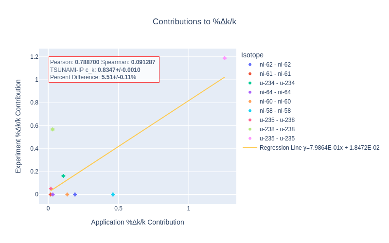
Fig. 1 An isotope-wise Plotly correlation plot between an experiment and application taken from the HMF series of critical experiments
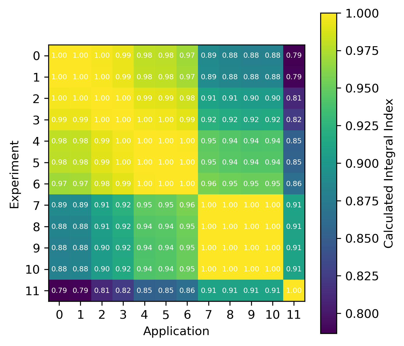

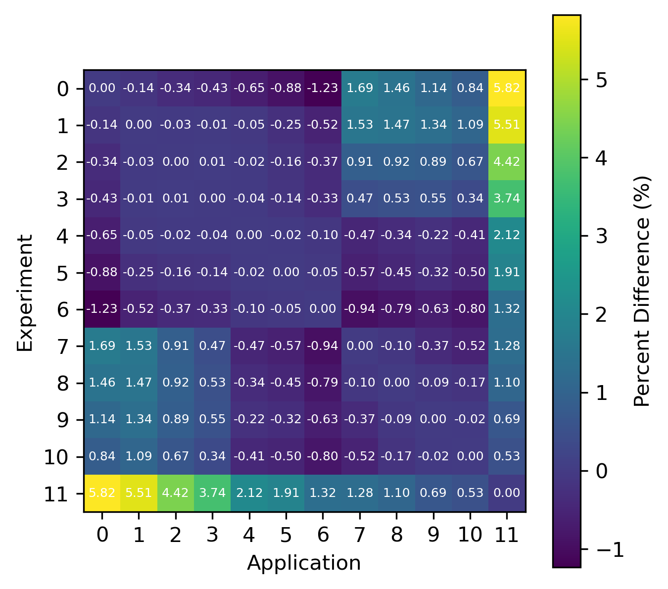

Fig. 2 Isotope-wise comparison of calculated correlation coefficients and TSUNAMI-IP \(c_k\) values for the HMF series of critical experiments [Bes19]
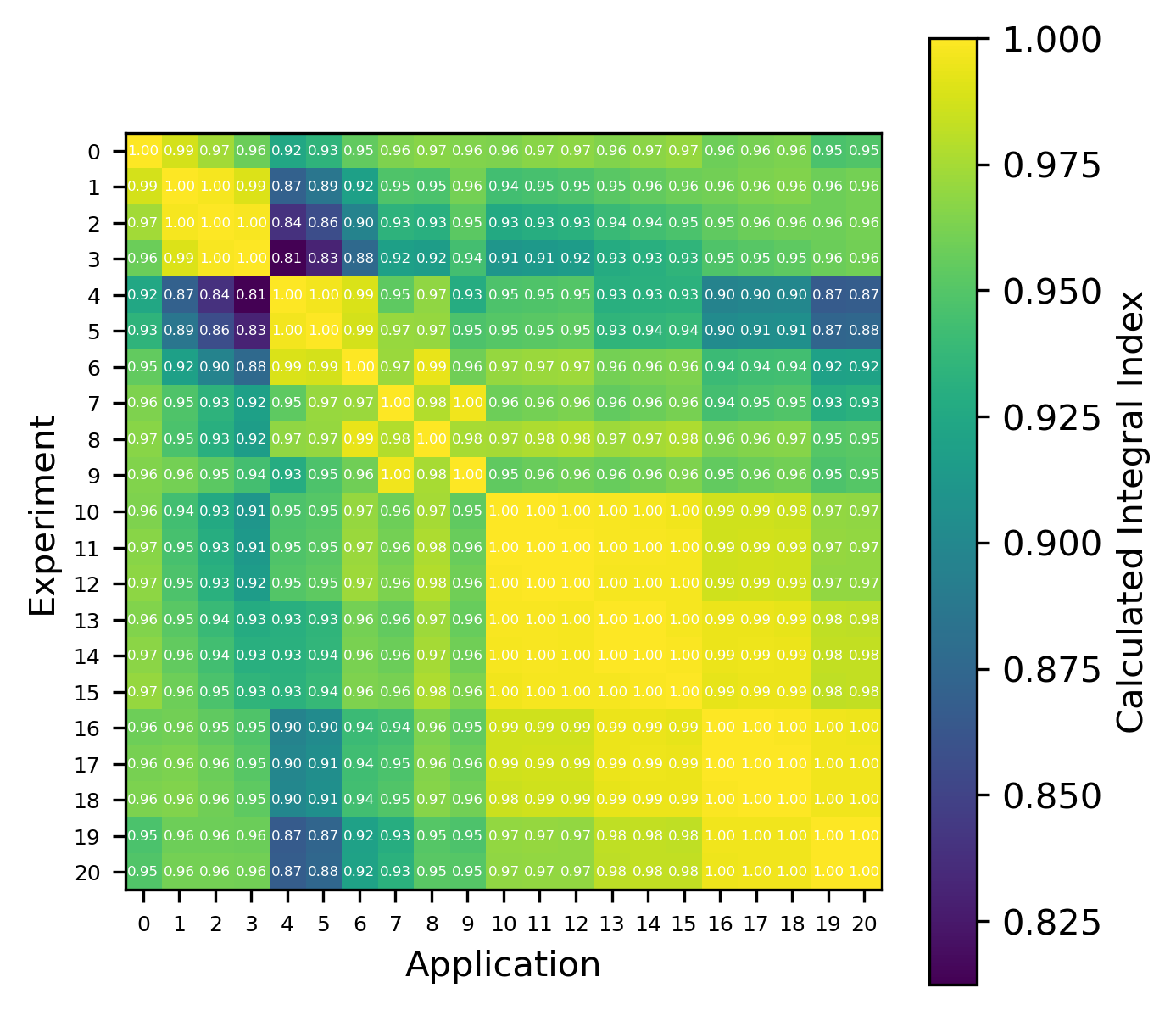

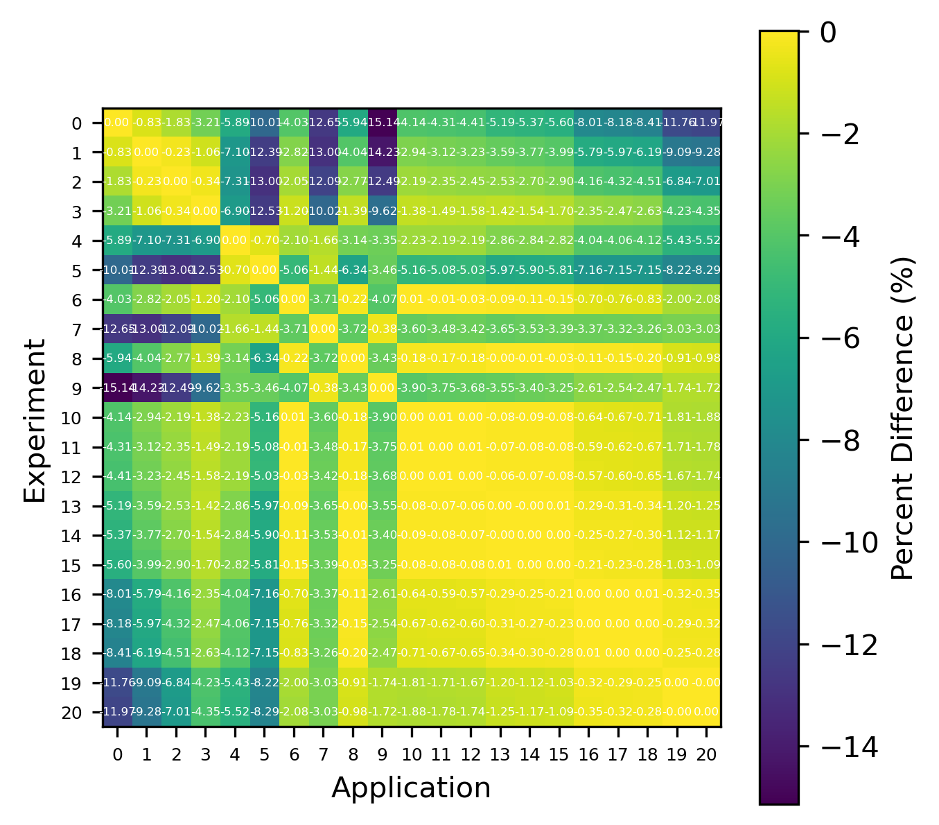

Fig. 3 Isotope-wise comparison of calculated correlation coefficients and TSUNAMI-IP \(c_k\) values for the MCT series of critical experiments [Bes19]
Isotope-Reaction–Wise
For reactions, the contribution correlation plots are as shown in Fig. 4. Again, several test cases were analyzed, and the results showing the difference in the calculated and TSUNAMI-IP \(c_k\) values are shown in Fig. 5 and Fig. 6. The results show good agreement except for the HMF cases, in which the errors are as large as 20%, and are not generally correlated with smaller \(c_k\).
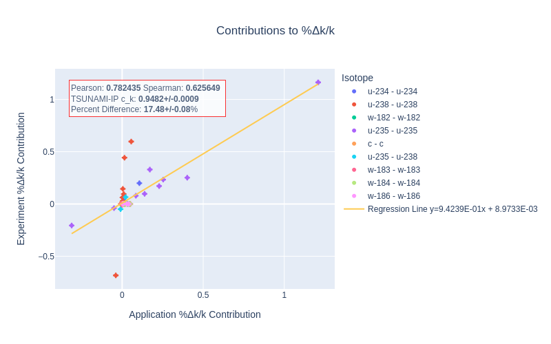
Fig. 4 A Reaction–wise Plotly correlation plot between an experiment and application taken from the HMF series of critical experiments
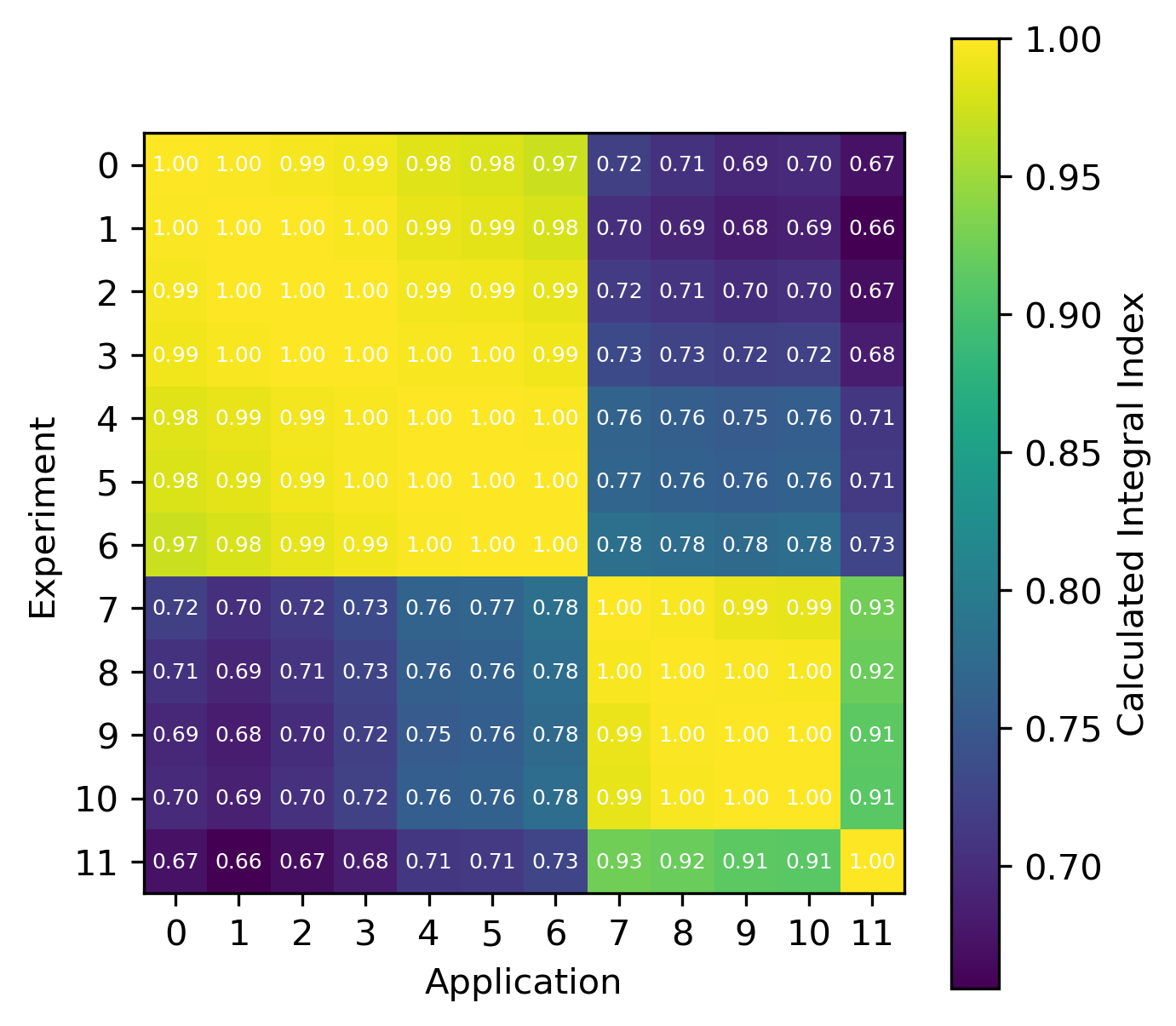
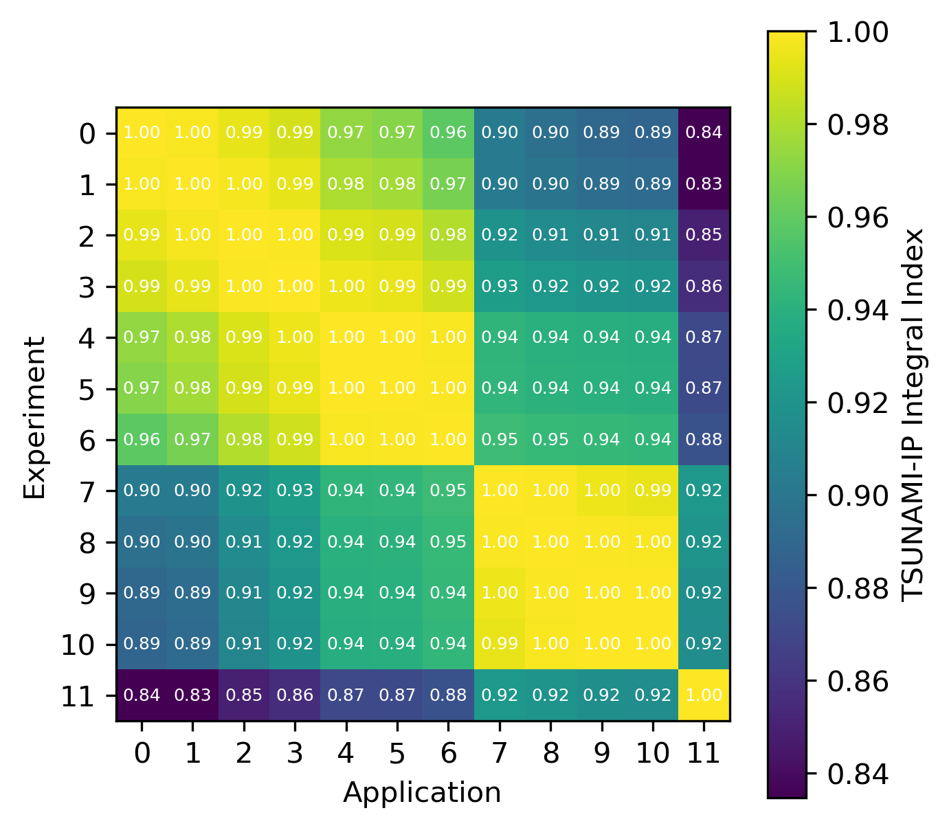
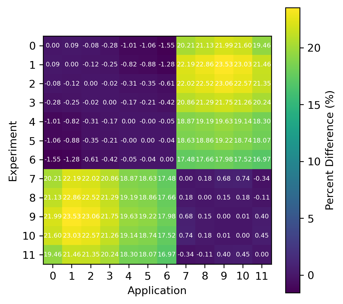

Fig. 5 Isotope-reaction-wise comparison of calculated correlation coefficients and TSUNAMI-IP \(c_k\) values for the HMF series of critical experiments [Bes19]
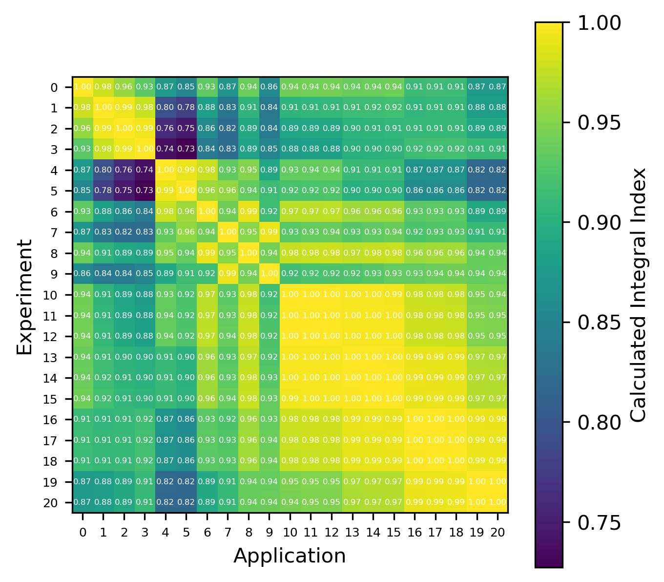
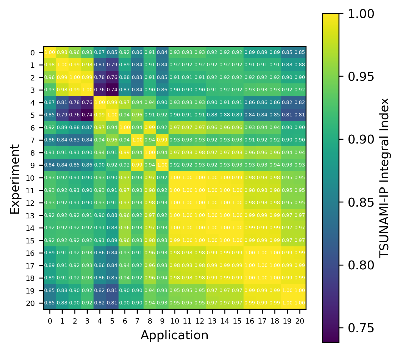
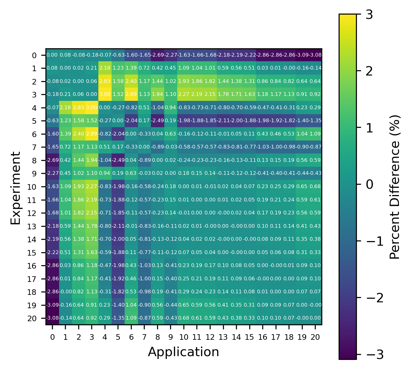

Fig. 6 Isotope-reaction-wise comparison of calculated correlation coefficients and TSUNAMI-IP \(c_k\) values for the MCT series of critical experiments [Bes19]
Consistent Random Variables
To find a method that better agrees with the calculated \(c_k\) value, a set of consistent random variables was selected with a correlation coefficient calculated with Eq. (2). One identified pair is given below:
where \(\boldsymbol{\sigma}\) is a row vector of length \(M\) representing the underlying nuclear data treated as a random variable, and \(\boldsymbol{S}_A\) and \(\boldsymbol{S}_B\) are row vectors containing the nuclide reaction and group-wise sensitivities for systems \(A\) and \(B\). Defining random variables in this way does not require Eq. (3) because the underlying random variables are known, and Eq. (2) can be used instead. This way, the formula for the correlation coefficient does not explicitly depend on the sample size \(N\) as in the previous case. First note that
Now, because \(\sigma_i\) and \(\sigma_j\) represent the group-wise cross section for a given nuclide reaction pair treated as a random variable, the following identification is possible:
The above expression for \(\text{Var}\left(X\right)\) can be written more succinctly as a matrix vector product with the covariance matrix: \(\boldsymbol{C}_{\alpha\alpha}\)
Likewise,
and
Substituting the above expressions into Eq. (2) gives
Relation to the Bias
Note that the variance and covariance of a random variable are invariant to constant shifts, as shown in Eq. (13), so the following pairs of random variables have the same correlation coefficient:
where \(\boldsymbol{\Delta \sigma}\) is a vector containing the differences of the cross sections from their mean values (e.g., those reported in the multigroup library used by SCALE). In this form, it is more apparent that random variables \(X\) and \(Y\) represent the perturbation in \(k\) as a result of random perturbations in the underlying cross-section data. That is, \(X=\Delta k_A\) and \(Y=\Delta k_B\), if they are viewed as random variables. This can be taken further by adding the mean \(k_{\text{eff}}\) reported by a transport code using the mean cross sections to both \(X\) and \(Y\), because it is simply a constant and does not change the correlation coefficient.
In other words, the random variables \(X\) and \(Y\) represent the \(k_{\text{eff}}\) of system \(A\) and \(B\) if they are treated as random variables (where the variation comes from variations in the underlying cross-section data). As a final step, assuming that for system \(A\) and \(B\), a true \(k_{\text{eff}}\) value exists, it can be subtracted from \(X\) and \(Y\) because, again, it is simply a constant:
This interpretation makes it clear that the reported correlation coefficient \(c_k\) represents the correlation of the biases between the two systems if viewed as random variables. This should be expected because, if the underlying nuclear data change for a given nuclide reaction pair as caused by measurement uncertainty (represented by \(\boldsymbol{\sigma}\) being treated as a random variable), then it will induce similar changes in the bias of system \(A\) and system \(B\) if they are correlated (if they depend similarly on the cross-section uncertainties), but this will not occur if the cause is not measurement uncertainty.
Implementation
To compute the correlation coefficient using the two random variables
defined above, it is necessary to sample from them and then compute the
sample Pearson correlation coefficient given in Eq.
(3). SCALE’s sampler utility
has the capability to randomly sample cross sections consistent with a
specified nuclear data and nuclear data covariance library. This utility
reads a set of statically generated cross-section perturbation factors
(1,000 samples total in SCALE 6.3
libraries [WL23]) and generates a perturbed
cross-section library which can then be read using standard AMPX
processing utilities [WL23]. To avoid having to
read and write perturbed cross-section libraries repeatedly for
different experiment application pairs, all of the perturbed libraries
were generated, read, and then cached as .pkl files. For a given
experiment application pair, the sensitivity data files are read,
\(\boldsymbol{S}_A\) and \(\boldsymbol{S}_B\) are generated, and
then the dot product is taken with a (cached) sampled perturbed
cross-section library to generate each point in the correlation plot, as
shown in Eq. (10).
Results
An example plot is presented in Fig. 7, showing near-agreement between the calculated and TSUNAMI-IP values. As before, the errors were calculated for a set of experiments, and the results are shown in Fig. 9 and Fig. 8. Despite the clean theoretical derivation in the previous section, the errors are very large (for the MCT cases, as high as 100%). The calculated errors are much larger than the sample standard deviation calculated by Eq. (4). For \(N=500\) and \(\rho=0.8\) (smaller \(\rho\) implies larger uncertainty, so \(\rho=0.8\) is conservative), \(\sigma_r\approx 0.016\), which implies a 2\(\sigma\) percent difference of \(\sim 4\%\), which is much smaller than the observed errors.
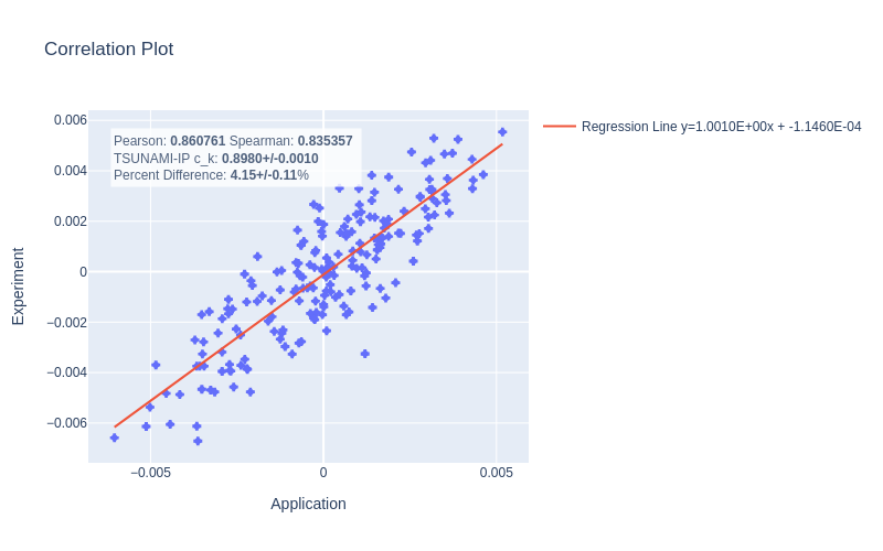
Fig. 7 A correlation plot generated using the variables defined in Eq. (10) for a given experiment application pair from the HMF series of critical experiments
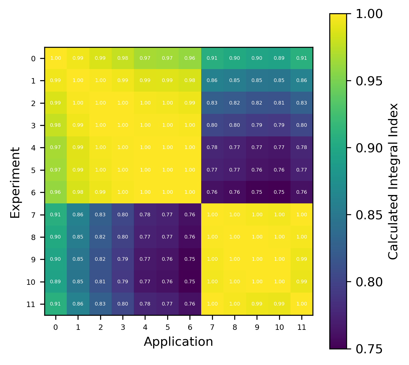
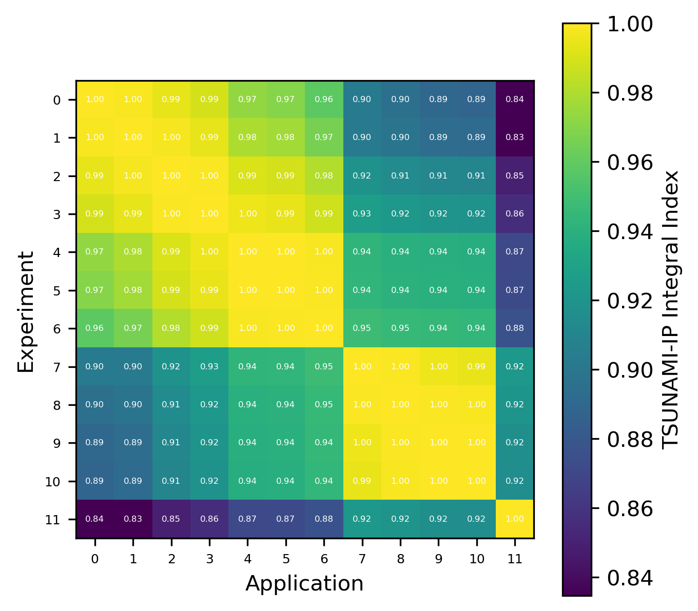
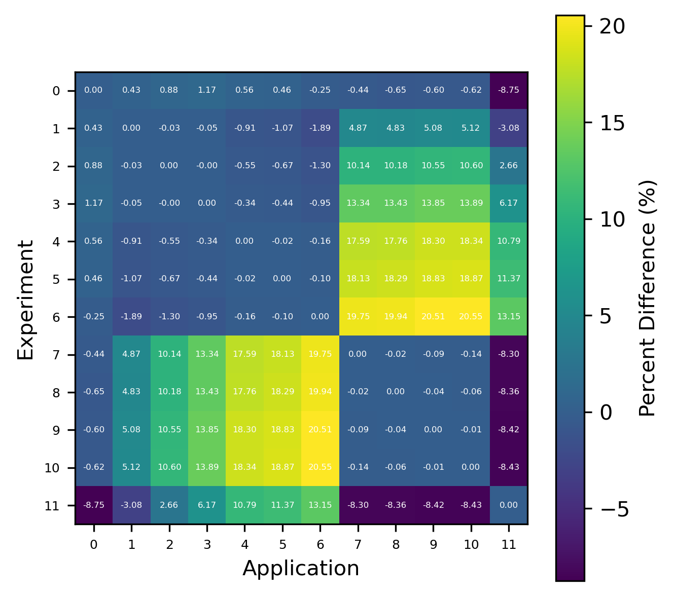

Fig. 8 Comparison of calculated correlation coefficients using the nuclear data sampling method (with 500 points) and TSUNAMI-IP \(c_k`\) values for the HMF series of critical experiments [Bes19]
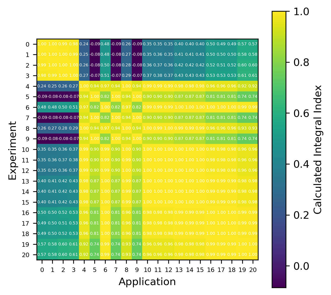

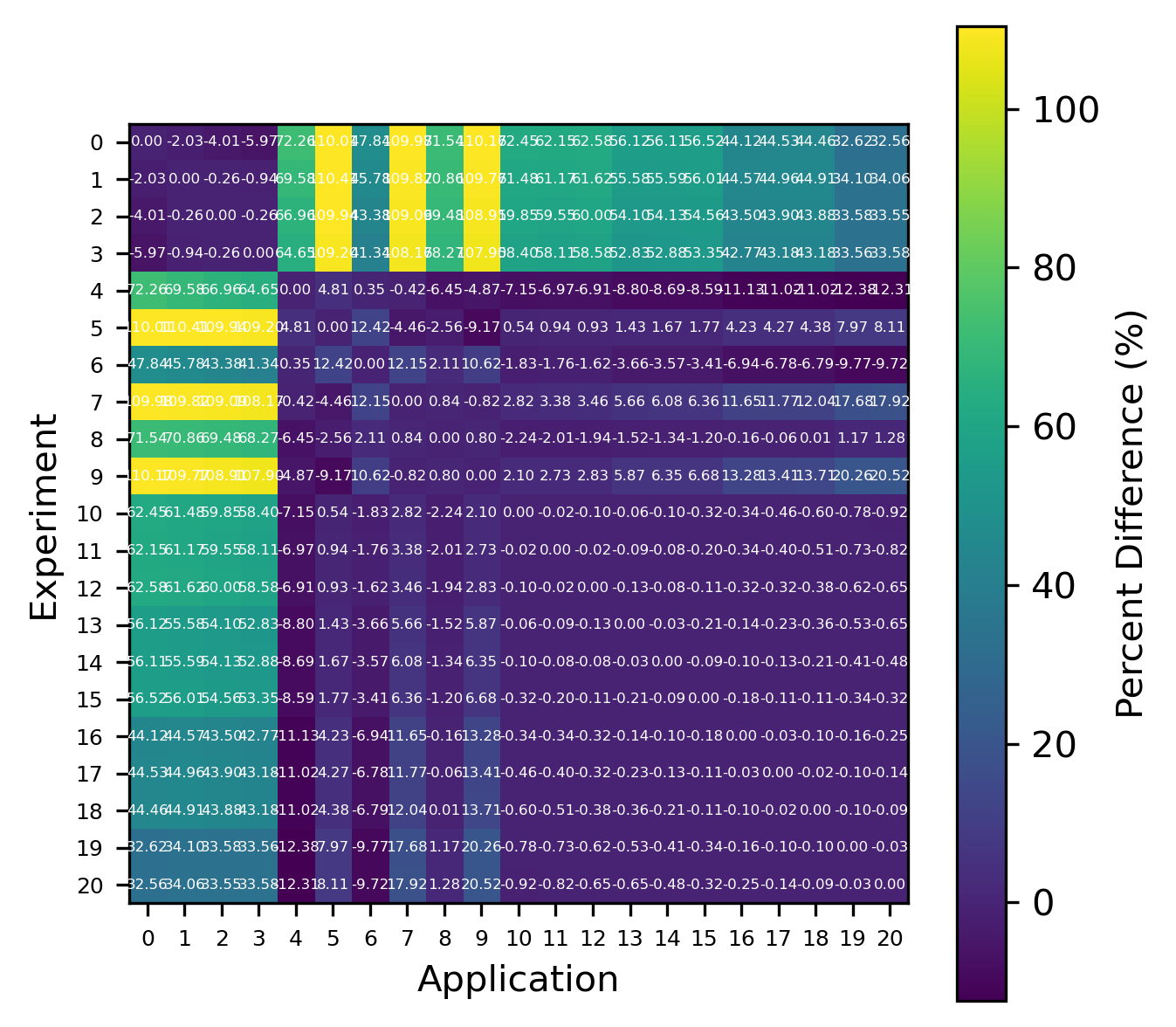

Fig. 9 Comparison of calculated correlation coefficients using the nuclear data sampling method (with 500 points) and TSUNAMI-IP \(c_k\) values for the MCT series of critical experiments [Bes19]
Future Work
The uncertainty contribution correlations shown in Section 3 may have better correspondence with the TSUNAMI-IP \(c_k\) if the full energy-dependent uncertainty contributions are used instead. When \(c_k\) is computed in TSUNAMI-IP, the full energy-dependent data are used, and in the energy integration, some data about system similarity are evidently lost. In general, a better mathematical understanding of the contribution correlations is required to understand its relation to \(c_k\).
In addition, the inconsistency with the nuclear data sampling method must be understood. It is possible that there is a subtle difference in how \(c_k\) is calculated in TSUNAMI-IP that’s causing the discrepancy. In any case, wildly different calculated correlations in cases like Fig. 10 need to be understood. In this case, not only is the correlation coefficient wrong in magnitude, but it is even wrong in direction. Also, the scales of the application and experiment are very different. If these values are truly to be interpreted as \(\Delta k\)s (as Section 4.1 would suggest), then the values of \(\pm 1\) shown in Fig. 10 are concerningly large and inconsistent with the calculated nuclear data–induced uncertainty of \(\sim 1-5\%\).(i.e., a \(\Delta k\) of \(\pm 1\) from nuclear data–induced uncertainty is several orders of magnitude larger than the reported standard deviation, which is impossibly unlikely). There may also be a discrepancy with how redundant reactions (e.g., “total” or “capture” in SCALE) are handled in TSUNAMI-IP. This idea could further be evaluated by explicitly computing \(k_{\text{eff}}\) for a system and application subject to randomly sampled cross sections using SCALE’s sampler routine [WL23].
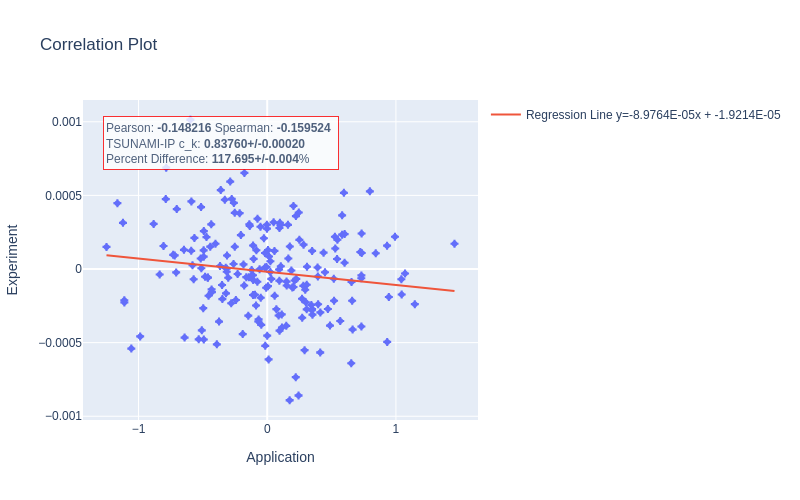
Fig. 10 An MCT case with exceptionally large disagreement with the TSUNAMI-IP calculated \(c_k\)
If these discrepancies can be better understood and/or eliminated, then these methods will provide a faithful (or at least heuristic) interpretation of \(c_k\) and may be the first step on the path to gaining a better understanding of which experiments are truly appropriate for code validation.
Acknowledgments
This work was supported in part by the US Department of Energy, Office of Science, Office of Workforce Development for Teachers and Scientists (WDTS) under the Science Undergraduate Laboratory Internships Program (SULI).
J Bess. International handbook of evaluated criticality safety benchmark experiments (icsbep). Organization for Economic Co-operation and Development-Nuclear Energy Agency Report NEA/NSC/DOC (95), 2019.
Douglas G Bowen and Nicholas W Brown. ANSI/ANS-8.1: Nuclear Criticality Safety in Operations with Fissile Material Outside Reactors. Transactions of the American Nuclear Society, 99:436–436, 2008.
BL Broadhead. Sensitivity and Uncertainty Analyses Applied to Criticality Safety Validation: Methods Development. US Nuclear Regulatory Commission, 1999.
Bryan L Broadhead, Bradley T Rearden, CM Hopper, JJ Wagschal, and CV Parks. Sensitivity- and Uncertainty-Based Criticality Safety Validation Techniques. Nuclear Science and Engineering, 146(3):340–366, 2004.
Elias Dabbas. Interactive Dashboards and Data Apps with Plotly and Dash: Harness the Power of a Fully Fledged Frontend Web Framework in Python–No JavaScript Required. Packt Publishing Ltd, 2021.
Lisa Fassino, Mathieu N Dupont, Iyad Al-Qasir, William A Wieselquist, and William BJ Marshall. Current State of Benchmark Applicability for Commercial-Scale HALEU Fuel Transport. 2024. URL: https://www.nrc.gov/docs/ML2410/ML24107A030.pdf.
Timo Gnambs. A Brief Note on the Standard Error of the Pearson Correlation. Collabra: Psychology, 2023.
Shane Hart and Justin Clarity. Creation of the VADER Code in SCALE. Technical Report, Oak Ridge National Laboratory (ORNL), Oak Ridge, TN (United States), 2022.
Harold Hotelling. The Impact of RA Fisher on Statistics. Journal of the American Statistical Association, 46(253):35–46, 1951.
Harold Hotelling. New Light on the Correlation Coefficient and Its Transforms. Journal of the Royal Statistical Society. Series B (Methodological), 15(2):193–232, 1953.
Henry Hurwitz. Note on a Theory of Danger Coefficients. General Electric Company, Knolls Atomic Power Laboratory, 1948.
Brian C Kiedrowski. Adjoint Weighting for Continuous-Energy Monte Carlo Radiation Transport. 2009.
William J Marshall, Justin B Clarity, and Bradley T Rearden. A Review of TSUNAMI Applications. Transactions of the American Nuclear Society, 2020.
Don Mueller, Bradley T Rearden, and Daniel F Hollenbach. Application of the SCALE TSUNAMI Tools for the Validation of Criticality Safety Calculations Involving $^233$U. 2 2009. URL: https://www.osti.gov/biblio/950002, doi:10.2172/950002.
Christopher M Perfetti and Bradley T Rearden. SCALE 6.2 Continuous-Energy TSUNAMI-3D Capabilities. Technical Report, Oak Ridge National Laboratory (ORNL), Oak Ridge, TN (United States), 2015.
Christopher Michael Perfetti. Advanced Monte Carlo methods for Eigenvalue Sensitivity Coefficient Calculations. PhD thesis, University of Michigan, 2012.
Ellen Marie Saylor, Alex Lang, William B. J. Marshall, and Robert Hall. Analysis of the 30B UF6 Container for Use with Increased Enrichment. 5 2021. URL: https://www.osti.gov/biblio/1797631, doi:10.2172/1797631.
John M Scaglione, Don E Mueller, and John C Wagner. An Approach for Validating Actinide and Fission Product Burnup Credit Criticality Safety Analyses: Criticality (k$_eff$) Predictions. Nuclear Technology, 188(3):266–279, 2014.
D Wiarda, ME Dunn, NM Greene, ML Williams, C Celik, and LM Petrie. AMPX-6: A Modular Code System for Processing ENDF/B. ORNL/TM-2016/43, 2016.
William Wieselquist and Robert Alexander Lefebvre. SCALE 6.3.1 User Manual. 2 2023. URL: https://www.osti.gov/biblio/1959594, doi:10.2172/1959594.
Relevant Identities
Variance of an Arbitrary Linear Combination of Random Variables
which is the form often given in textbooks.
Bilinearity of the Covariance
The covariance is linear in one argument at a time:
Shift Independence of Variance
For a random variable \(X\), the variance of a shifted random variable \(Y=X-a\) is the same: